I often use Twitter as a place to vent about the horribleness of Excel, from the product itself to analyses its UI and workflow influences. Admittedly, some of this is snobbish preference: if everyone used my preferred tools, then the world would be a better place! But let me back off my snobbishness a bit and just say this: please feel free to use any tool you want, up to and including pencil-and-paper…JUST.STOP.USING.EXCEL.

Excel arbitrarily destroys data for fun, as evidenced by the example below.

Who Gives A ‘F’ About Seconds? I’m 10 minutes Late Everywhere!

CSV files have many flaws, but at least they are just plain text. It doesn’t take any special software to read them and you can open and close them without loss of fidelity…except if you open them with Excel.

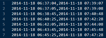
Suppose you have a CSV file with timestamps in ISO8601 format. Depending on which text editor you use, it might look something like this:

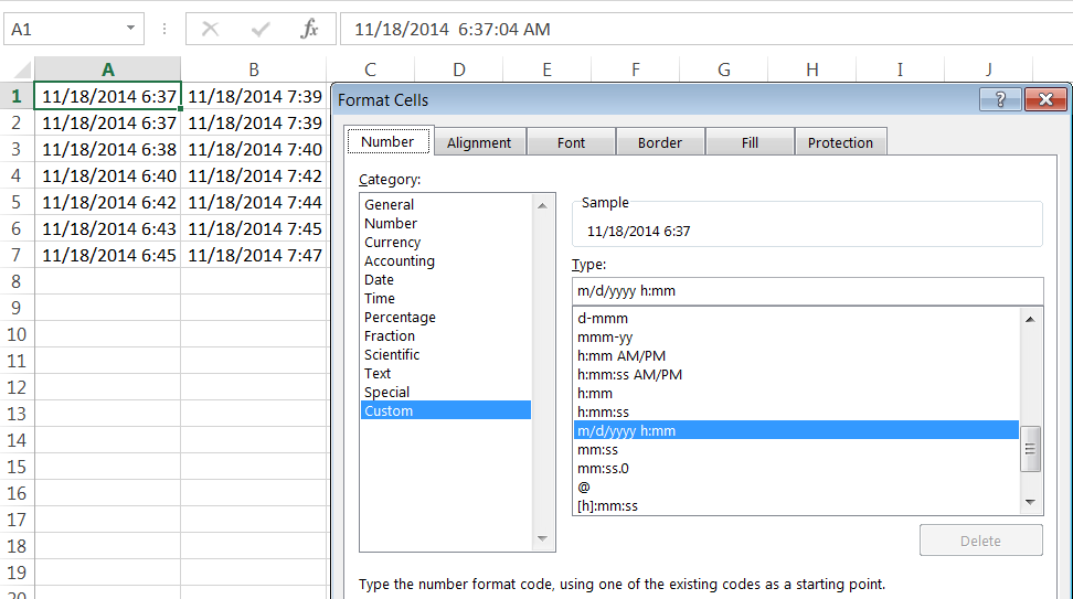
Now, let’s open our file in Excel:

The first thing you might notice is that not only does Excel change the date formatting in the file to be more “‘Murica!”, they don’t even have the courtesy to use one of their existing date or time formats! And rather than keep the date the way it was, or standardize the dates to the way the rest of the world writes them, or even keep fixed-width columns, Excel feels like it should also hide the seconds! Makes sense…seconds are for other people to see, if/when they highlight an individual cell.

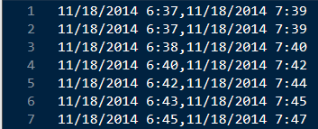
So, you’ve opened this file, but can’t remember if you made any changes outside of applying auto-width to the columns. The data still looks right, so you hit ‘Save’ when prompted by Excel. But you remember that your favorite programmer asked for a CSV file, and it’s already a CSV file, so you hit save, ignore the ‘features’ Excel brags about and email it back to your co-worker. Here’s what they receive:

Reading this back in our plain-text editor, we can now see we have a loss of fidelity of between 37 and 47 seconds on each cell of data. Whereas Excel keeps track of your timestamps while you’re in a SPREADSHEET, if you save as plain text, Excel assumes you want to keep the format it automatically applied to your data (automatically! silently!), and thus, destroys your file. In what world would you not care about seconds in your timestamps?

Remember, this mis-feature occurs even if the only thing you do is open a plain-text file in Excel and hit save. No other Excel actions are needed to destroy your data.

Excel: Only The Proper Tool If You Don’t Care

If you don’t care about using the proper tool for analytics, don’t want to learn something new, don’t want numerical accuracy, hate visually interesting graphics, don’t need reproducibility…use Excel. For everything else, there’s everything else. Don’t be a VLOOKUP guru, use SQL. Don’t store your data in Excel just because it allows for a million rows, use a database. If you need point-and-click graphics, at least spring for Tableau so the defaults look nicer.

Or, learn to code using open-source languages for a total licensing cost of $0. Every analyst would get value from knowing one open-source analytics language, even topically, so that you can write simple calculation scripts and document your thought process. A side benefit is that by coding, you can also use version control like Git or SVN. Then, you can have different versions of thought, and the next analyst down the line can see how your analysis has evolved.

And while I’m ranting, a special message for all you ‘top-tier’ analytics consultants out there: you should know SEVERAL of the common analytics languages. If you do your “analysis” in Excel, you are a hack or you are just providing reporting for $300/hr. Use better tools, your clients deserve better. I have infinitely more respect for someone who delivers a sloppy set of slides and a documented R script than someone who knows who to put drop-shadows on MS Office documents and makes fancy decks. You are being judged not just by the C-Suite, but also by snobs like me. And when contract renewal time comes around, they do ask my opinion and I do make comments on how sophisticated your toolset was that you used (or lack thereof if you’re using Excel).

It’s nearly 2015, do better. Stop Using Excel.

It’s been nearly a year since I wrote Twitter.jl, back when I seemingly had MUCH more free time. In these past 10 months, I’ve used Julia quite a bit to develop other packages, and I try to use it at work when I know I’m not going to be collaborating with others (since my colleagues don’t know Julia, not because it’s bad for collaboration!).

One of the things that’s obvious from my earlier Julia code is that I didn’t understand how powerful metaprogramming can be, so here’s a simple example where I can replace 50 lines of Julia code with 10.

CTRL-A, CTRL-C, CTRL-P. Repeat.

Admittedly, when I started on the Twitter package, I fully meant to go back and clean up the codebase, but moved onto something more fun instead. The Twitter package started out as a means of learning how to use the Requests.jl library to make API calls, figure out the OAuth syntax I needed (which itself should be factored out of Twitter.jl), then copied-and-pasted the same basic function structure over and over. While fast, what I was left with was this (currently, the help.jl file in the Twitter package):

1
2
3
4
5
6
7
8
9
10
11
12
13
14
15
16
17
18
19
20
21
22
23
24
25
26
27
28
29
30
31
32
33
34
35
36
37
38
39
40
41
42
43
44
45
#############################################################
#
# Help section Functions for Twitter API
#
#############################################################

function get_help_configuration(; options=Dict{String, String}())

    r = get_oauth("https://api.twitter.com/1.1/help/configuration.json", options)

    return r.status == 200 ? JSON.parse(r.data) : r

end

function get_help_languages(; options=Dict{String, String}())

    r = get_oauth("https://api.twitter.com/1.1/help/languages.json", options)

    return r.status == 200 ? JSON.parse(r.data) : r

end

function get_help_privacy(; options=Dict{String, String}())

    r = get_oauth("https://api.twitter.com/1.1/help/privacy.json", options)

    return r.status == 200 ? JSON.parse(r.data) : r

end

function get_help_tos(; options=Dict{String, String}())

    r = get_oauth("https://api.twitter.com/1.1/help/tos.json", options)

    return r.status == 200 ? JSON.parse(r.data) : r

end

function get_application_rate_limit_status(; options=Dict{String, String}())

    r = get_oauth("https://api.twitter.com/1.1/application/rate_limit_status.json", options)

    return r.status == 200 ? JSON.parse(r.data) : r

end

It’s pretty clear that this is the same exact code pattern, right down to the spacing! The way to interpret this code is that for these five Twitter API methods, there are no required inputs. Optionally, there is the ‘options’ keyword that allows for specifying a Dict() of options. For these five functions, there are no options you can pass to the Twitter API, so even this keyword is redundant. These are simple functions so I don’t gain a lot by way of maintainability by using metaprogramming, but at the same time, one of the core tenets of programming is ‘Don’t Repeat Yourself’, so let’s clean this up.

For :symbol in symbolslist…

In order to clean this up, we need to take out the unique parts of the function, then pass them as arguments to the @eval macro as follows:

1
2
3
4
5
6
7
8
9
10
11
12
funcname = (:get_help_configuration, :get_help_languages, :get_help_privacy, :get_help_tos, :get_application_rate_limit_status)
endpoint = ("help/configuration.json", "help/languages.json", "help/privacy.json",  "help/tos.json", "application/rate_limit_status.json")

for (func, endp) in zip(funcname, endpoint)
	@eval function ($func)(; options=Dict{String, String}())

	        r = get_oauth($"https://api.twitter.com/1.1/$endp", options)

	        return r.status == 200 ? JSON.parse(r.data) : r

    	end
end

What’s happening in this code is that I define two tuples: one of function names (as symbols, denoted by :) and one of the API endpoints. We can then iterate over the two tuples, substituting the function names and endpoints into the code. When the package is loaded, this code evaluates, defining the five functions for use in the Twitter package.

Wha?

Yeah, so metaprogramming can be simple, but it can also be mind-bending. It’s one thing to not repeat yourself, it’s another to write something so complex that even YOU can’t remember how the code works. But somewhere in between lies a sweet spot where you can re-factor whole swaths of code and streamline your codebase. Metaprogramming is used throughout the Julia codebase, so if you’re interested in seeing more examples of metaprogramming, check out the Julia source code, the Requests.jl package (where I first saw this) or really anyone who actually knows what they are doing. I’m just a metaprogramming pretender at this point 🙂  

To read additional discussion around this specific example, see the Julia-Users discussion at: https://groups.google.com/forum/#!topic/julia-users/zvJmqB2N0GQ

Edit, 11/22/2014: DarthToaster on Reddit provided another fantastic way to approach refactoring, using macros:

1
2
3
4
5
6
7
8
9
10
11
macro endpoint(name, path)
    quote
        function $(esc(name))(; options=Dict{String, String}())
            r = get_oauth($"https://api.twitter.com/1.1/$path", options)
            return r.status == 200 ? JSON.parse(r.data) : r
        end
    end
end

@endpoint get_help_configuration "help/configuration.json"
@endpoint get_help_languages "help/languages.json"

Changes

Version 1.4.1 of RSiteCatalyst is now available on CRAN. There were a handful of bug fixes and new features added, including:

• Fixed bug in QueueRanked function where only 10 results were returned when requesting multiple element reports. Function now returns up to 50,000 per breakdown (API limit)
• Created better error message to inform user to login with credentials instead of making function call without proper API credentials
• Added support for using SAINT classifications in QueueRanked/QueueTrended functions
• Added more error checking to make functions fail more elegantly
• Added remaining GET methods from Reporting/Administration API

Additional GET methods

This version of RSiteCatalyst has roughly 20 new GET methods, mostly providing additional report suite information for those who might desire to generate their documentation programmatically rather than manually. New API methods include (but are not limited to):

• GetMarketingChannelRules: Get a list of all criteria used to build the Marketing Channels report
• GetReportDescription: For a given bookmark_id, get the report definition
• GetListVariables: Get a list of the List Variables defined for a report suite
• GetLogins: Get all logins for a given Company

If you were the type of person who enjoyed this blog post showing how to auto-generate Adobe Analytics documentation, I encourage you to take a look at these newly incorporated functions and use them to improve your documentation even further.

Feature Requests/Bugs

If you come across any bugs, or have any feature requests, please continue to use the RSiteCatalyst GitHub Issues page to make tickets. While I’ve responded to many of you via the maintainer email provided in the R package itself, it’s much more efficient (and you’re much more likely to get a response) if you use the GitHub Issues page. Don’t worry about cluttering up the page with tickets, please fill out a new issue for anything you encounter, unless you are SURE that it is the same problem someone else is facing.

And finally, like I end every blog post about RSiteCatalyst, please note that I’m not an Adobe employee. Please don’t send me your API credentials, expect immediate replies or ask to set up phone calls to troubleshoot your problems. This is open-source software…Willem Paling and I did the hard part writing it, you’re expected to support yourself as best as possible unless you believe you’re encountering a bug. Then use GitHub 🙂