“Well, first you need a TMS and a three-tiered data layer, then some jQuery with a node backend to inject customer data into the page asynchronously if you want to avoid cookie-based limitations with cross-domain tracking and be Internet Explorer 4 compatible…”
Blah Blah Blah. There’s a whole cottage industry around jargon-ing each other to death about digital data collection. But why? Why do we focus on tools, instead of the data? Because the tools are necessarily inflexible, so we work backwards from the pre-defined reports we have to the data needed to populate them correctly. Let’s go the other way for once: clickstream data to analysis & reporting.
In this blog post, I will show the structure of the Adobe Analytics Clickstream Data Feed and how to work with a day worth of data within R. Clickstream data isn’t as raw as pure server logs, but the only limit to what we can calculate from clickstream data is what we can accomplish with a bit of programming and imagination. In later posts, I’ll show how to store a year worth of data in a relational database, storing the same data in Hadoop and doing analysis using modern tools such as Apache Spark.
This blog post will not cover the mechanics of getting the feed delivered via FTP. The Adobe Clickstream Feed documentation is sufficiently clear in how to get started.
FTP/File Structure
Once your Adobe Clickstream Feed starts being delivered via FTP, you’ll have a file listing that looks similar to the following:
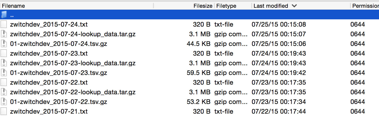
What you’ll notice is that with daily delivery, three files are provided, each having a consistent file naming format:
- \d+-\S+_\d+-\d+-\d+.tsv.gz
This is the main file containing the server call level data
- \S+_\d+-\d+-\d+-lookup_data.tar.gz
These are the lookup tables, header files, etc.
- \S+_\d+-\d+-\d+.txt
Manifest file, delivered last so that any automated processes know that Adobe is finished transferring
The regular expressions will be unnecessary for working with our single day of data, but it’s good to realize that there is a consistent naming structure.
Checking md5 hashes
As part of the manifest file, Adobe provides md5 hashes of the files. There are at least two purposes to this, including 1) making sure that the files truly were delivered in full and 2) that the files haven’t been manipulated/tampered with. In order to check that your md5 hashes match the values provided by Adobe, we can do the following in R:
1
2
3
4
5
6
7
8
9
10
11
12
13
14
setwd("~/Downloads/datafeed/")

#Read in Adobe manifest file
manifest <- read.table("zwitchdev_2015-07-13.txt", stringsAsFactors=FALSE)
names(manifest) <- c("key", "value")

#Use digest library to calculate md5 hashes
library(digest)
servercalls_md5 <- digest("01-zwitchdev_2015-07-13.tsv.gz", algo="md5", file=TRUE)
lookup_md5 <- digest("zwitchdev_2015-07-13-lookup_data.tar.gz", algo="md5", file=TRUE)

#Check to see if hashes contained in manifest file
servercalls_md5 %in% manifest$value #[1] TRUE
lookup_md5 %in% manifest$value #[1] TRUE
As we can see, both calculated hashes are contained within the manifest, so we can be confident that the files we downloaded haven’t been modified.
Unzipping and Loading Raw Files to Data Frames
Now that our file hashes are validated, it’s time to load the files into R. For the example files, I would be able to fit the entire day into RAM because my blog does very little traffic. However, I’m going to still limit the rows brought in, as if we were working with a large e-commerce website with millions of visits per day:
1
2
3
4
5
6
7
8
9
10
11
12
13
14
15
16
17
18
19
20
21
22
23
24
25
26
#Get list of lookup files from tarball
files_tar <- untar("zwitchdev_2015-07-13-lookup_data.tar.gz", list = TRUE)

#Extract files to _temp directory. Directory will be created if it doesn't exist
untar("zwitchdev_2015-07-13-lookup_data.tar.gz", exdir = "_temp")

#Read each file into a data frame
#If coding like this in R offends you, keep it to yourself...
for (file in files_tar) {
  df_name <- unlist(strsplit(file, split = ".tsv", fixed = TRUE))
  temp_df <- read.delim(paste("_temp", file, sep = "/"), header=FALSE, stringsAsFactors=FALSE)
  #column_headers not used as lookup table
  if (df_name != "column_headers"){
    names(temp_df) <- c("id", df_name)
  }
  assign(df_name, temp_df)
  rm(temp_df)
}

#gz files can be read directly into dataframes from base R
#Could also use `readr` library for performance
servercall_data <- read.delim("~/Downloads/datafeed/01-zwitchdev_2015-07-13.tsv.gz",
                       header=FALSE, stringsAsFactors=FALSE, nrows = 500)

#Use column_headers to label servercall_data data frame using first row of data
names(servercall_data) <- column_headers[1,]
If we were to be loading this data into a database, we’d be done with our processing; we have all of our data read into R and it would be a trivial exercise to load the data into a database (we’ll do this in a separate blog post). But since we’re going to be analyze this single day of clickstream data, we need to join these 14 data frames together.
SQL: The Most Important Language for Analytics
As a slight tangent, if you don’t know SQL, then you’re going to have a really hard time doing any sort of advanced analytics. There are literally millions of tutorials on the Internet (including this one from me), and understanding how to join and retrieve data from databases is the key to being more than just a report monkey.
The reason why the prior code creates 14 data frames is because the data is delivered in a normalized structure from Adobe. Now we are going to de-normalize the data, which is just a fancy way of saying “join the files together in order to make a gigantic table.”
There are probably a dozen different ways to join data frames using just R code, but I’m going to do it using the sqldf package so that I can use SQL. This will allow for a single, declarative statement that shows the relationship between the lookup and fact tables:
1
2
3
4
5
6
7
8
9
10
11
12
13
14
15
16
17
18
19
20
21
22
23
24
25
26
27
28
29
30
library(sqldf)

query <-
"select
sc.*,
browser.browser as browser_name,
browser_type,
connection_type.connection_type as connection_name,
country.country as country_name,
javascript_version,
languages.languages as languages,
operating_systems,
referrer_type,
resolution.resolution as screen_resolution,
search_engines
from servercall_data as sc
left join browser on sc.browser = browser.id
left join browser_type on sc.browser = browser_type.id
left join connection_type on sc.connection_type = connection_type.id
left join country on sc.country = country.id
left join javascript_version on sc.javascript = javascript_version.id
left join languages on sc.language = languages.id
left join operating_systems on sc.os = operating_systems.id
left join referrer_type on sc.ref_type = referrer_type.id
left join resolution on sc.resolution = resolution.id
left join search_engines on sc.post_search_engine = search_engines.id
;
"

denormalized_df <- sqldf(query)
There are three lookup tables that weren’t used: color_depth, plugins and event. The first two don’t have a lookup column in my data feed (click link for a full listing of Adobe Clickstream data feed columns available). These columns aren’t really useful for my purposes anyway, so not a huge loss. The third table, the event list, requires a separate processing step.
Processing Event Data
As normalized as the Adobe Clickstream Data Feed is, there is one oddity: the events per server call come in a comma-delimited string in a single column with a lookup table. This implies that a separate level of processing is necessary, outside of SQL, since the column “key” is actually multiple keys and the lookup table specifies one event type per row. So if you were to try and join the data together, you wouldn’t get any matches.
To deal with this in R, we are going to do an EXTREMELY wasteful operation: we are going to create a data frame with a column for each possible event, then evaluate each row to see if that event occurred. This will use a massive amount of RAM, but of course, this is a feature/limitation of R which wouldn’t be an issue if the data were stored in a database.
1
2
3
4
5
6
7
8
9
10
11
12
13
14
15
16
17
18
19
20
21
22
23
#Create friendly names in events table replacing spaces with underscores
event$names_filled <- tolower(gsub(" ", "_", event$event))

#Initialize a data frame with all 0 values
#Dimensions are number of observations as rows, with a column for every possible event
event_df <- data.frame(matrix(data = 0, ncol = nrow(event), nrow = nrow(servercall_data)))
names(event_df) <- event$id

#Parse comma-delimited string into vector
#Each vector value represents column name in event_df, assign value of 1
for(row in servercall_data$post_event_list){
    if(!is.na(row)){
        for(event_ in strsplit(row, ",")){
          event_df[as.character(event_)] <- 1
        }
    }
}

#Rename columns with "friendly" names
names(event_df) <- event$names_filled

#Horizontally join datasets to create final dataset
oneday_df <- cbind(denormalized_df, event_df)
With the final cbind command, we’ve created a 500 row x 1562 column dataset representing a sample of rows from one day of the Adobe Clickstream Data Feed. Having the data denormalized in this fashion takes 6.13 MB of RAM…extrapolating to 1 million rows, you would need 12.26GB of RAM (per day of data you want to analyze, if stored solely in memory).
Next Step: Analytics?!
A thousand words in and 91 lines of R code and we still haven’t done any actual analytics. But we’ve completed the first step in any analytics project: data prep!
In future blog posts in this series, I’ll demonstrate how to actually use this data in analytics, from re-creating reports available in the Adobe Analytics UI (to prove the data is the same) to more advanced analysis such as using association rules, which can be one method for creating a “You may also like…” functionality such as the one at the bottom of this blog.