As digital marketers & analysts, we’re often asked to quantify when a metric goes beyond just random variation and becomes an actual “unexpected” result. In cases such as A/B..N testing, it’s easy to calculate a t-test to quantify the difference between two testing populations, but for time-series metrics, using a t-test is likely not appropriate.
To determine whether a time-series has become “out-of-control”, we can use Exponential Smoothing to forecast the Expected Value, as well as calculate Upper Control Limits (UCL) and Lower Control Limits (LCL). To the extent a data point exceeds the UCL or falls below the LCL, we can say that statistically a time-series is no longer within the expected range. There are numerous ways to create time-series models using R, but for the purposes of this blog post I’m going to focus on Exponential Smoothing, which is how the anomaly detection feature is implemented within the Adobe Analytics API.
Holt-Winters & Exponential Smoothing
There are three techniques that the Adobe Analytics API uses to build time-series models:
- Holt-Winters Additive (Triple Exponential Smoothing)
- Holt-Winters Multiplicative (Triple Exponential Smoothing)
- Holt Trend Corrected (Double Exponential Smoothing)
The formulas behind each of the techniques are easily found elsewhere, but the main point behind the three techniques is that time-series data can have a long-term trend (Double Exponential Smoothing) and/or a seasonal trend (Triple Exponential Smoothing). To the extent that a time-series has a seasonal component, the seasonal component can be additive (a fixed amount of increase across the series, such as the number of degrees increase in temperature in Summer) or multiplicative (a multiplier relative to the level of the series, such as a 10% increase in sales during holiday periods).
The Adobe Analytics API simplifies the choice of which technique to use by calculating a forecast using all three methods, then choosing the method that has the best fit as calculated by the model having the minimum (squared) error. It’s important to note that while this is probably an okay model selection method for detecting anomalies, this method does not guarantee that the model chosen is the actual “best” forecast model to fit the data.
RSiteCatalyst API call
Using the RSiteCatalyst R package version 1.1, it’s trivial to access the anomaly detection feature:
1
2
3
4
5
6
7
8
9
10
11
12
#Run until version > 1.0 on CRAN
library(devtools)
install_github("RSiteCatalyst", "randyzwitch", ref = "master")

#Run if version >= 1.1 on CRAN
library("RSiteCatalyst")

#API Authentication
SCAuth(<username:company>, <shared_secret>)

#API function call
pageviews_w_forecast <- QueueOvertime(reportSuiteID=<report suite>, dateFrom = "2013-06-01", dateTo="2013-08-13", metrics = "pageviews", dateGranularity="day", anomalyDetection="1")
Once the function call is run, you will receive a DataFrame of ‘Day’ granularity with the actual metric and three additional columns for the forecasted value, UCL and LCL. Graphing these data using ggplot2 (Graph Code Here - GitHub Gist), we can now see on which days an anomalous result occurred:
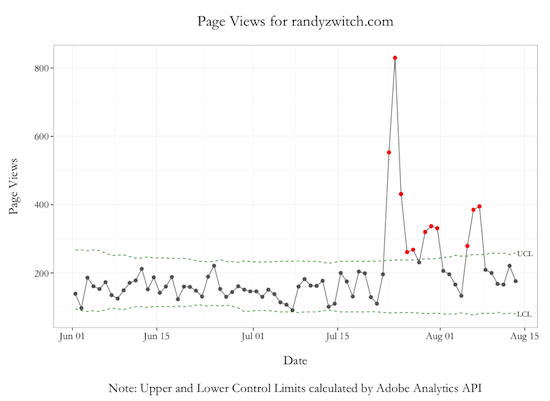
The red dots in the graph above indicate days where page views either exceeded the UCL or fell below the LCL. On July 23 - 24 timeframe, traffic to this blog spiked dramatically due to a blog post about the Julia programming language, and continued to stay above the norm for about a week afterwards.
Anomaly Detection Limitations
There two limitations to keep in mind when using the Anomaly Detection feature of the Adobe Analytics API:
- Anomaly Detection is currently only available for ‘Day’ granularity
- Forecasts are built on 35 days of past history
In neither case do I view these limitations as dealbreakers. The first limitation is just an engineering decision, which I’m sure could be expanded if enough people used this functionality.
For the time period of 35 days to build the forecasts, this is an area where there is a balance between calculation time vs. capturing a long-term and/or seasonal trend in the data. Using 35 days as your time period, you get five weeks of day-of-week seasonality, as well as 35 points to calculate a ‘long-term’ trend. If the time period is of concern in terms of what constitutes a ‘good forecast’, then there are plenty of other techniques that can be explored using R (or any other statistical software for that matter).
Elevating the discussion
I have to give a hearty ‘Well Done!’ to the Adobe Analytics folks for elevating the discussion in terms of digital analytics. By using statistical techniques like Exponential Smoothing, analysts can move away from qualitative statements like “Does it look like something is wrong with our data?” to actually quantifying when KPIs are “too far” away from the norm and should be explored further.