Last week, I wrote a blog post showing how to sessionize log data using standard SQL. The main idea of that post is that if your analytics platform supports window functions (like Postgres and Hive do), you can make quick work out of sessionizing logs. Here’s the winning query:

1
2
3
4
5
6
7
8
9
10
11
12
13
14
15
select
uid,
sum(new_event_boundary) OVER (PARTITION BY uid ORDER BY event_timestamp) as session_id,
event_timestamp,
minutes_since_last_interval,
new_event_boundary
from
			--Query 1: Define boundary events
			(select
			uid,
			event_timestamp,
			(extract(epoch from event_timestamp) - lag(extract(epoch from event_timestamp)) OVER (PARTITION BY uid ORDER BY event_timestamp))/60 as minutes_since_last_interval,
			case when extract(epoch from event_timestamp) - lag(extract(epoch from event_timestamp)) OVER (PARTITION BY uid ORDER BY event_timestamp) > 30 * 60 then 1 ELSE 0 END as new_event_boundary
			from single_col_timestamp
			) a;

One nested sub-query and two window functions are all it takes to calculate the event boundaries and create a unique identifier for sessions for any arbitrary timeout chosen.

It’s Hadley’s House, We’re Just Leasing

Up until today, I hadn’t really done anything using dplyr.  But having a bunch of free time this week and hearing people talk so much about how great dplyr is, I decided to see what it would take to replicate this same exercise using R. dplyr has support for Postgres as a back-end, and has verbs that translate R code into window functions, so I figured it had to be possible. Here’s what I came up with:

1
2
3
4
5
6
7
8
9
10
11
12
13
14
15
16
17
18
19
20
21
22
23
24
25
26
27
28
29
###Sessionization using dplyr

library(dplyr)

#Open a localhost connection to Postgres
#Use table 'single_col_timestamp'
#group by uid and sort by timestamp for window function
#Do minutes calculation, working around missing support for extract(epoch from timestamp)
#Calculate event boundary and unique id via cumulative sum window function
sessions <-  
        src_postgres("logfiles") %>%
        tbl("single_col_timestamp") %>%
        group_by(uid) %>%
        arrange(event_timestamp) %>%
        mutate(minutes_since_last_event = (
                                           DATE_PART('day', event_timestamp - lag(event_timestamp)) * 24 +
                                           DATE_PART('hour', event_timestamp - lag(event_timestamp)) * 60 +
                                           DATE_PART('minute', event_timestamp - lag(event_timestamp)) * 60 +
                                           DATE_PART('second', event_timestamp - lag(event_timestamp))
                                           ) / 60
              ) %>%
        mutate(event_boundary = if(minutes_since_last_event > 30) 1 else 0,
               session_id = order_by(event_timestamp, cumsum(if(minutes_since_last_event > 30) 1 else 0)))

#Show query syntax
show_query(sessions)

#Actually run the query
answer <- collect(sessions)

Generally, I’m not a fan of the pipe operator, but I figured I’d give it a shot since everyone else seems to like it. This is one nasty bit of R code, but ultimately, it is possible to get the same result as writing SQL directly. I did need to take a few roundabout ways, specifically in calculating the minutes between timestamps and substituting the CASE expression into the window function rather than call it by name, but it’s basically the same logic.

Why Does This Work?

If you compare the SQL code above to the R code, you might be wondering why the dplyr code works. Certainly, working the dplyr way gives me cognitive dissonance, as you generally specify the verbs you are using in reverse order as you do in SQL. But calling show_query(sessions), you actually see that dplyr is generating SQL under-the-hood (I formatted the code for easier viewing):

1
2
3
4
5
6
7
8
9
10
11
12
13
14
15
16
17
18
19
20
21
22
23
24
25
26
SELECT
	"uid",
	"event_timestamp",
	"minutes_since_last_event",
	"event_boundary",
	"session_id"
FROM (
		SELECT
			"uid",
			"event_timestamp",
			"minutes_since_last_event",
			CASE WHEN "minutes_since_last_event" > 30.0 THEN 1.0 ELSE 0.0 END AS "event_boundary",
			sum(CASE WHEN "minutes_since_last_event" > 30.0 THEN 1.0 ELSE 0.0 END) OVER (PARTITION BY "uid" ORDER BY "event_timestamp" ROWS UNBOUNDED PRECEDING) AS "session_id"
		FROM
			(
				SELECT
					"uid",
					"event_timestamp",
					(DATE_PART('day', "event_timestamp" - LAG("event_timestamp", 1, NULL) OVER (PARTITION BY "uid" ORDER BY "event_timestamp")) * 24.0
						+ DATE_PART('hour', "event_timestamp" - LAG("event_timestamp", 1, NULL) OVER (PARTITION BY "uid" ORDER BY "event_timestamp")) * 60.0
						+ DATE_PART('minute', "event_timestamp" - LAG("event_timestamp", 1, NULL) OVER (PARTITION BY "uid" ORDER BY "event_timestamp")) * 60.0
						+ DATE_PART('second', "event_timestamp" - LAG("event_timestamp", 1, NULL) OVER (PARTITION BY "uid" ORDER BY "event_timestamp"))) / 60.0 AS "minutes_since_last_event"
				FROM "single_col_timestamp"
				ORDER BY "uid", "event_timestamp"
			) AS "_W1"
	) AS "_W2"

Like all SQL-generating tools, the code is a bit inelegant; however, I have to say that I’m truly impressed the dplyr code was able to handle this scenario at all, given that this example has to be at least an edge-, if not a corner-case of what dplyr is meant for in terms of data manipulation.

So, dplyr Is Going To Become Part Of Your Toolbox?

While it was possible to re-create the same functionality, ultimately, I don’t see myself using dplyr a whole lot. In the case of using databases, it seems more efficient and portable just to write the SQL directly; at the very least, it’s what I’m already comfortable doing as part of my analytics workflow. For manipulating data frames, maybe I’d use it (I do use plyr extensively in my RSiteCatalyst package), but I’d probably be more inclined to use sqldf instead.

But that’s just me, not a reflection on the package quality. Happy manipulating, however you choose to do it! 🙂

Over my career as a predictive modeler/data scientist, the most important step(s) in any data project without question have been data cleaning and feature engineering. By taking the data you have, correcting flaws and reformulating raw data into additional business-specific concepts, you ensure that you move beyond pure mathematical optimization and actually solve a business problem. While “big data” is often held up as the future of knowing everything, when it comes down to it, a Hadoop cluster is more often a “Ha-dump” cluster: the place data gets dumped without any proper ETL.

For this blog post, I’m going to highlight a common request for time-series data: combining discrete events into sessions. Whether you are dealing with sensor data, television viewing data, digital analytics data or any other stream of events, the problem of interest is usually how a human interacts with a machine over a given period of time, not each individual event.

While I usually use Hive (Hadoop) for daily work, I’m going to use Postgres (via OSX Postgres.app) to make this as widely accessible as possible. In general, this process will work with any infrastructure/SQL-dialect that supports window functions.

Connecting to Database/Load Data

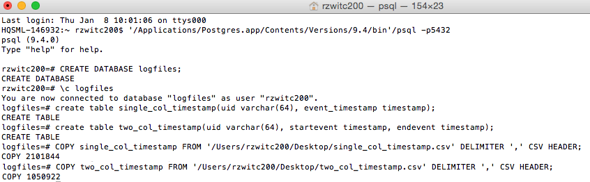
For lightweight tasks, I find using psql (command-line tool) is easy enough. Here are the commands to create a database to hold our data and to load our two .csv files (download here and here):

These files contain timestamps generated for 1000 uid values.

Query 1 (“Inner”): Determining Session Boundary Using A Window Function

In order to determine the boundary of each session, we can use a window function along with lag(), which will allow the current row being processed to compare vs. the prior row. Of course, for all of this to work correctly, we need to have our data sorted in time order by each of our users:

1
2
3
4
5
6
7
--Create boundaries at 30 minute timeout
select
uid,
event_timestamp,
(extract(epoch from event_timestamp) - lag(extract(epoch from event_timestamp)) OVER (PARTITION BY uid ORDER BY event_timestamp))/60 as minutes_since_last_interval,
case when extract(epoch from event_timestamp) - lag(extract(epoch from event_timestamp)) OVER (PARTITION BY uid ORDER BY event_timestamp) > 30 * 60 then 1 ELSE 0 END as new_event_boundary
from single_col_timestamp;

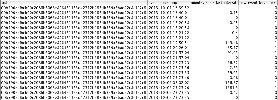
For this query, we use the lag() function on the event_timestamp column, and we use over partition by uid order by event_timestamp to define the window over which we want to do our calculation. To provide additional clarification about how this syntax works, I’ve added a column showing how many minutes have passed between intervals to validate that the 30-minute window is calculated correctly. The result is as follows:

For each row where the value of minutes_since_last_interval > 30, there is a value of 1 for new_event_boundary.

Query 2 (“Outer”): Creating A Session ID

The query above defines the event boundaries (which is helpful), but if we want to calculate session-level metrics, we need to create a unique id for each set of rows that are part of one session. To do this, we’re again going to use a window function:

1
2
3
4
5
6
7
8
9
10
11
12
13
14
15
select
uid,
sum(new_event_boundary) OVER (PARTITION BY uid ORDER BY event_timestamp) as session_id,
event_timestamp,
minutes_since_last_interval,
new_event_boundary
from
			--Query 1: Define boundary events
			(select
			uid,
			event_timestamp,
			(extract(epoch from event_timestamp) - lag(extract(epoch from event_timestamp)) OVER (PARTITION BY uid ORDER BY event_timestamp))/60 as minutes_since_last_interval,
			case when extract(epoch from event_timestamp) - lag(extract(epoch from event_timestamp)) OVER (PARTITION BY uid ORDER BY event_timestamp) > 30 * 60 then 1 ELSE 0 END as new_event_boundary
			from single_col_timestamp
			) a;

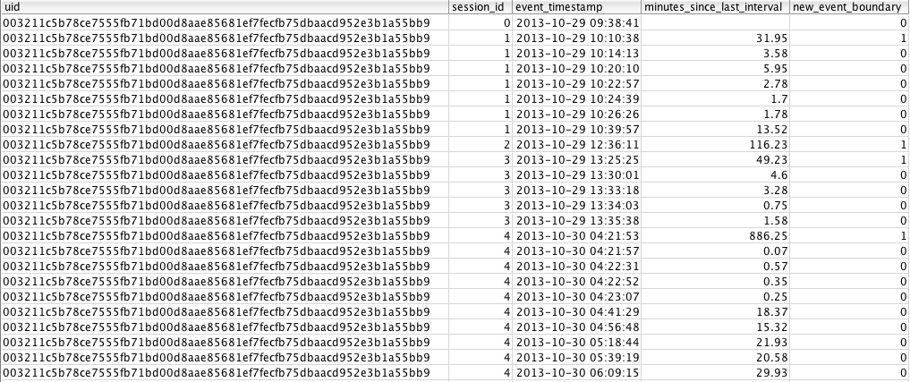
This query defines the same over partition by uid order by event_timestamp window, but rather than using lag() this time, we’re going to use sum() for the outer query. The effect of using sum() in our window function is to do a cumulative sum; every time 1 shows up, the session_id field gets incremented by 1. If there is a value of 0, the sum is still the same as the row above and thus has the same session_id. This is easier to understand visually:

At this point, we have a session_id for a group of rows where there have been no 30 minute gaps in behavior.

Final Query: Cleaned Up

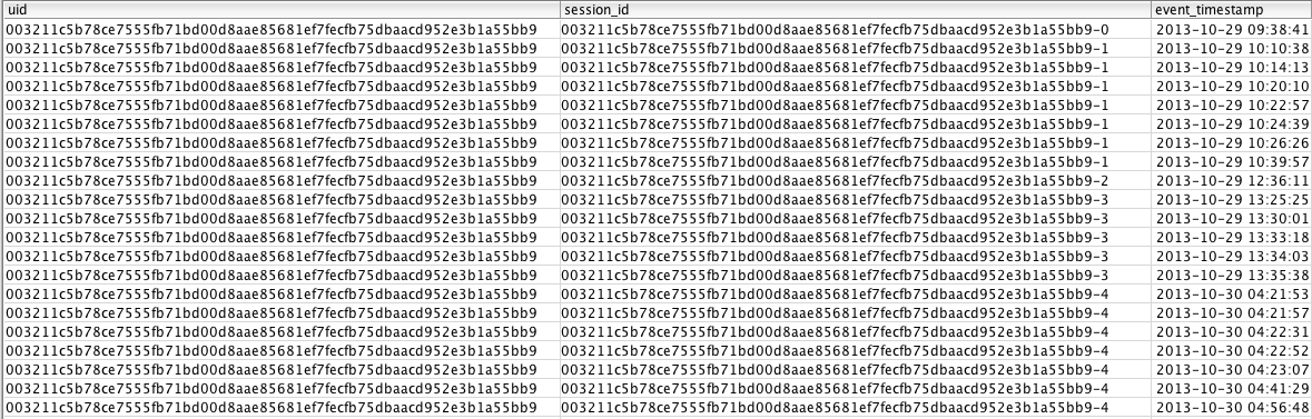
Although the previous section is technically done, I usually concatenate the uid and session_id together.  I do this concatenation just to highlight that the value is usually a ‘key’ value, not a metric in itself (though it can be). Concatenating the keys together and removing the teaching columns results in the following query:

1
2
3
4
5
6
7
8
9
10
11
12
13
--Query 3:  Outer query uses window function with sum to do cumulative sum as the id, concatentate to uid
select
uid,
uid || '-' || cast(sum(new_event_boundary) OVER (PARTITION BY uid ORDER BY event_timestamp) as varchar) as session_id,
event_timestamp
from
			--Query 1: Define boundary events
			(select
			uid,
			event_timestamp,
			case when extract(epoch from event_timestamp) - lag(extract(epoch from event_timestamp)) OVER (PARTITION BY uid ORDER BY event_timestamp) > 30 * 60 then 1 ELSE 0 END as new_event_boundary
			from single_col_timestamp
			) a;

Window Functions, Will You Marry Me?

The first time I was asked to try and solve sessionization of time-series data using Hive, I was sure the answer would be that I’d have to get a peer to write some nasty custom Java code to be able generate unique ids; in retrospect, the solution is so obvious and simple that I wish I would’ve tried to do this years ago. This is a pretty easy problem to solve using imperative programming, but if you’ve got a gigantic amount of hardware in a RDBMS or Hadoop, SQL takes care of all of the calculation without needing think through looping (or more complicated logic/data structures).

Window functions fall into a weird space in the SQL language, given that they allow you to do sequential calculations when SQL should generally be thought of as “set-level” calculations (i.e. no implied order and table-wide calculations vs. row/state-specific). But now that I’ve got a hang of them, I can’t imagine my analytical life without them.

It’s a new year, so…new version of RSiteCatalyst on CRAN! For the most part, this release fixes a handful of bugs that weren’t noticed with the prior release 1.4.2 (oops!), but there are pieces of additional functionality.

New functionality: Data Feed monitoring

For those of you having hourly or daily data feeds delivered via FTP, you can now find out the details of a data feed and all of a company’s feeds & the processing status of each using GetFeed() and GetFeeds() respectively.

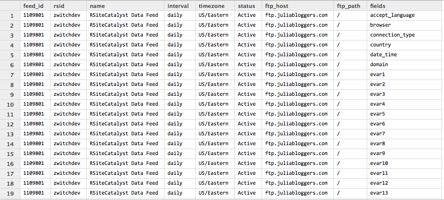
For example, calling GetFeed() with a specific feed number will return the following information as a data frame:

Similarly, if you call GetFeeds("report-suite"), you’ll get the following information as a data frame:

I only have one feed set up for testing, but if there were more feeds delivered each day, they would show up as additional rows in the data frame. The interpretation here is that the daily feed for 1/5/15 was delivered (the 05:00:00 is GMT).

Bug Fixes

RSiteCatalyst v1.4.2 attempted to fix an issue where QueueRanked would error if two SAINT classifications were used. Unfortunately, by fixing that issue, QueueRanked ONLY worked with SAINT Classifications. This was only out in the wild for a month, so hopefully it didn’t really affect anyone.

Additionally, the segment.id and segment.name weren’t printing out to the data frame in the Queue* functions. This has also been fixed.

Test Suite Using Travis CI

To avoid future errors like the ones mentioned above, a full test suite using testthat has been added to RSiteCatalyst and monitored via Travis CI. While there is coverage for every public function within the package, there are likely additional tests that can be added for functionality I didn’t cover. If anyone out there has particularly weird cases they use and aren’t incorporated in the test suite, please feel free to file an issue or submit a pull request and I’ll figure out how to incorporate it into the test suite.

DataWarehouse API

Finally, the last bit of changes to RSiteCatalyst in v1.4.3 are internal preparations for a new package I plan to release in the coming months: AdobeDW. Several folks have asked for the ability to control Data Warehouse reports via R; for various reasons, I thought it made sense to break this out from RSiteCatalyst into its own package. If there are any R-and-Adobe-Analytics enthusiasts out there that would like to help development, please let me know!

Feature Requests/Bugs

As always, if you come across bugs or have feature requests, please continue to use the RSiteCatalyst GitHub Issues page to submit issues. Don’t worry about cluttering up the page with tickets, please fill out a new issue for anything you encounter (with code you’ve already tried and is failing), unless you are SURE that it is the same problem someone else is facing.

And finally, like I end every blog post about RSiteCatalyst, please note that I’m not an Adobe employee. This hasn’t been an issue for a few months, so maybe next time I won’t end the post with this boilerplate :)