Recently I’ve been spending a lot of time trying to learn Julia by doing the problems at Project Euler. What’s great about these problems is that it gets me out of my normal design patterns, since I don’t generally think about prime numbers, factorials and other number theory problems during my normal workday. These problems have also given me the opportunity to really think about how computers work, since Julia allows the programmer to pass type declarations to the just-in-time compiler (JIT).

As I’ve been working on optimizing my Julia code, I decided to figure out how fast this problem can be solved using any of the languages/techniques I know. So I decided to benchmark one of the Project Euler problems using Julia, Python, Python with Numba, PyPy, R, R using the compiler package, pqR and pqR using the compiler package. Here’s what I found…

Problem

The problem I’m using for the benchmark is calculating the smallest number that is divisible by all of the numbers in a factorial. For example, for the numbers in 5!, 60 is the smallest number that is divisible by 2, 3, 4 and 5. Here’s the Julia code:

1
2
3
4
5
6
7
8
9
10
11
function smallestdivisall(n::Int64)
    for i = 1:factorial(n)
        for j = 1:n
            if i % j !=0
                break
            elseif j == n
                return i
            end
        end
    end
end

All code versions follow this same pattern: the outside loop will run from 1 up to n!, since by definition the last value in the loop will be divisible by all of the numbers in the factorial. The inner loops go through and do a modulo calculation, checking to see if there is a remainder after division. If there is a remainder, break out of the loop and move to the next number. Once the state occurs where there is no remainder on the modulo calculation and the inner loop value of j equals the last number in the factorial (i.e. it is divisible by all of the factorial numbers), we have found the minimum number.

Benchmarking - Overall

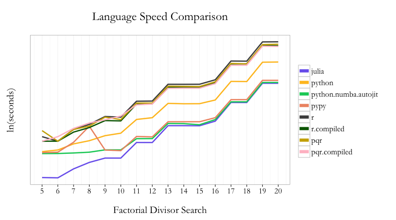
Here are the results of the eight permutations of languages/techniques (see this GitHub Gist for the actual code used, this link for results file, and this GitHub Gist for the ggplot2 code):

Across the range of tests from 5! to 20!, Julia is the fastest to find the minimum number. Python with Numba is second and PyPy is third. pqR fares better than R in general, but using the compiler package can narrow the gap.

To make more useful comparisons, in the next section I’ll compare each language to its “compiled” function state.

Benchmarking - Individual

Python

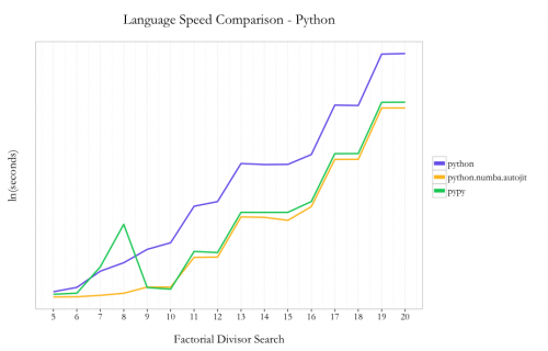
Amongst the native Python code options, I saw a 16x speedup by using PyPy instead of Python 2.7.6 (10.62s vs. 172.06s at 20!). Using Numba with Python instead of PyPy nets an incremental ~40% speedup using the @autojit decorator (7.63s vs. 10.63 at 20!).

So in the case of Python, using two lines of code with the Numba JIT compiler you can get substantial improvements in performance without needing to do any code re-writes. This is a great benefit given that you can stay in native Python, since PyPy doesn’t support all existing packages within the Python ecosystem.

R/pqR

It’s understood in the R community that loops are not a strong point of the language. In the case of this problem, I decided to use loops because 1) it keeps the code pattern similar across languages and 2) I hoped I’d see the max benefit from the compiler package by not trying any funky R optimizations up front.

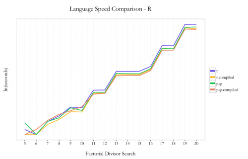
As expected, pqR is generally faster than R and using the compiler package is faster than not using the compiler. I saw ~30% improvement using pqR relative to R and ~20% incremental improvement using the compiler package with pqR. Using the compiler package within R showed ~35% improvement.

So unlike the case with Python, where you could just use Python with Numba and stay within the same language/environment, if you can use pqR and the compiler package, you can get a performance benefit from using both.

Summary

For a comparison like I’ve done above, it’s easy to get carried away and extrapolate the results from one simple test to all programming problems ever. “Julia is the best language for all cases ever!!!11111eleventy!” would be easy to proclaim, but all problems aren’t looping problems using simple division. Once you get into writing longer programs, other tasks such string manipulation and accessing APIs, using a technique from a package only available in one ecosystem but not another, etc., which tool is “best” for solving a problem becomes a much more difficult decision. The only way to know how much improvement you can see from different techniques & tools is to profile your program(s) and experiment.

The main thing that I took away from this exercise is that no matter which tool you are comfortable with to do analysis, there are potentially large performance improvements that can be made just by using a JIT without needing to dramatically re-write your code. For those of us who don’t know C (and/or are too lazy to re-write our code several times to wring out a little extra performance), that’s a great thing.

RSiteCatalyst version 1.1 is now available on CRAN. Changes from version 1 include:

• Support for Correlations/Subrelations in the QueueRanked function
• Support for Current Data in all Queue* functions
• Support Anomaly Detection for QueueOvertime and QueueTrended functions (example usage with ggplot2 graph)
• Decrease in wait time for API calls (from 5 seconds to 2 seconds) and extending total number of API tries before report failure (from 100 seconds to 10 minutes)

For those of you Adobe Analytics (Omniture) users who haven’t yet tried to use the Adobe Analytics API, I’ve created an introduction video to get started. There will also continue to be examples of using this package on this blog on the RSiteCatalyst tag. Enjoy!

In the previous three tutorials (1, 2, 3), we’ve covered the background of Hadoop, how to build a proof-of-concept Hadoop cluster using Amazon EC2 and how to upload a .zip file to the cluster using Hue. In Part 4, we’ll use the data uploaded from the .zip file to create a master table of all files, as well as creating a view.

Creating Tables Using Hive

Like SQL for ‘regular’ relational databases, Hive is the tool we can use within Hadoop to create tables from data loaded into HDFS. Because Hadoop was built with large, messy data in mind, there are some amazingly convenient features for creating and loading data, such as being able to load all files in a directory (assuming they have the same format).  Here’s the Hive statement we can use to load the airline dataset:

1
2
3
4
5
6
7
8
9
10
11
12
13
14
15
16
17
18
19
20
21
22
23
24
25
26
27
28
29
30
31
32
33
34
35
36
-- Create table from yearly airline csv files
CREATE EXTERNAL TABLE airline (
  `Year` int,
  `Month` int,
  `DayofMonth` int,
  `DayOfWeek` int,
  `DepTime`  int,
  `CRSDepTime` int,
  `ArrTime` int,
  `CRSArrTime` int,
  `UniqueCarrier` string,
  `FlightNum` int,
  `TailNum` string,
  `ActualElapsedTime` int,
  `CRSElapsedTime` int,
  `AirTime` int,
  `ArrDelay` int,
  `DepDelay` int,
  `Origin` string,
  `Dest` string,
  `Distance` int,
  `TaxiIn` int,
  `TaxiOut` int,
  `Cancelled` int,
  `CancellationCode` string,
  `Diverted` string,
  `CarrierDelay` int,
  `WeatherDelay` int,
  `NASDelay` int,
  `SecurityDelay` int,
  `LateAircraftDelay` int)
ROW FORMAT DELIMITED
FIELDS TERMINATED BY ','
ESCAPED BY '\\'
STORED AS TEXTFILE
LOCATION '/user/hue/airline/airline';

The above statement starts by outlining the structure of the table, which is mostly integers with a few string columns. The next four lines of code specifies what type of data we have, which are delimited files where the fields are terminated (separated) by commas and where the delimiter is escaped using a backslash. Finally, we type the location of our files, which is the location of the directory where we uploaded the .zip file in part 3 of this tutorial. Note that we specify an “external table”, which means that if we drop the ‘airline’ table, we will still retain our raw data. Had we not specified the external keyword, Hive would’ve moved our raw data files into Hive, and had we decided to drop the ‘airline’ table, all our data would be deleted. Specifying external also lets us build multiple tables on the same underlying dataset if we so choose.

Creating a View Using Hive

One thing that’s slightly awkward above Hive is that you can’t specify that there is a header row in your files. As such, once the above code loads, we have 22 rows in our ‘airline’ table where the data is invalid. Another thing that’s awkward about Hive is that there is no row-level operations, so you can’t delete data! However, we can very easily fix our problem using a view:

1
2
3
4
-- Create view to "remove" 22 bad records from our table
create view vw_airline as
select * from airline
where uniquecarrier <> "UniqueCarrier";

Now that we have our view defined, we no longer have to explicitly exclude the rows in every future query we run. Just like in SQL, views are “free” from a performance standpoint, as they don’t require any additional data storage space (they just represent stored code references).

Time for Analysis?!

If you’ve made it this far, you’ve waited a long time to do some actual analysis! The next and final part of this tutorial will do some interesting things using Hive and/or Pig to analyze the data. The origin of this dataset was a data mining contest to predict why a flight would arrive late to its destination and we’ll do examples towards that end.