String Interpolation for Fun and Profit

Randy Zwitch × July 14, 2014 × DataScience

In a previous post, I showed how I frequently use Julia as a ‘glue’ language to connect multiple systems in a complicated data pipeline. For this blog post, I will show two more examples where I use Julia for general programming, rather than for computationally-intense programs.

String Building: Introduction

The Strings section of the Julia Manual provides a very in-depth treatment of the considerations when using strings within Julia. For the purposes of my examples, there are only three things to know:

Strings are immutable within Julia and 1-indexed
Strings are easily created through the a syntax familiar to most languages:

julia> authorname = "randy zwitch"
"randy zwitch"

julia> typeof(authorname)
String

String interpolation is easiest done using dollar-sign notation. Additionally, parenthesis can be used to avoid symbol ambiguity:

julia> interpolated = "the author of this blog post is $(authorname)"
"the author of this blog post is randy zwitch"

If you are using large volumes of textual data, you’ll want to pay attention to the difference between the various string types that Julia provides (UTF8/16/32, ASCII, Unicode, etc), but for the purposes of this blog post we’ll just be using the ASCIIString type by not explicitly declaring the string type and only using ASCII characters.

EDIT, 9/8/2016: Starting with version 0.5, Julia defaults to the String type, which is an UTF-8 character encoding.

Example 1: Repetitive Queries

As part of my data engineering responsibilities at work, I often get requests to pull a sample of every table in a new database in our Hadoop cluster. This type of request is usually from the business owner, who wants to evaluate the data set has been imported correctly, but doesn’t actually want to write any sort of queries. So using the ODBC.jl package, I repeatedly do the same select * from <tablename> query and save to individual .tab files:

1
2
3
4
5
6
7
8
9
10
11
12
13
14
15
16
17
18
19
20
21
22
_
_       _ _(_)_     |  A fresh approach to technical computing
(_)     | (_) (_)    |  Documentation: http://docs.julialang.org
_ _   _| |_  __ _   |  Type "help()" to list help topics
| | | | | | |/ _` |  |
| | |_| | | | (_| |  |  Version 0.3.0-prerelease+4028 (2014-07-02 23:42 UTC)
_/ |\__'_|_|_|\__'_|  |  Commit 2185bd1 (11 days old master)
|__/                   |  x86_64-w64-mingw32
julia> using ODBC
julia> ODBC.connect("Production hiveserver2", usr="", pwd="")
ODBC Connection Object
----------------------
Connection Data Source: Production hiveserver2
Production hiveserver2 Connection Number: 1
Contains resultset? No
julia> tables = query("show tables in db;");
elapsed time: 0.167028049 seconds
julia> for tbl in tables[:tab_name]
query("select * from db.$(tbl) limit 1000;"; output="C:\\data_dump\\$(tbl).tab", delim='\t')
end

julia>

While the query is simple, writing/running this hundreds of times would be a waste of effort. So with a simple loop over the array of tables, I can provide a sample of hundreds of tables in .tab files with five lines of code.

Example 2: Generating Query Code

In another task, I was asked to join a handful of Hive tables, then transpose the table from “long” to “wide”, so that each id value only had one row instead of multiple. This is fairly trivial to do using CASE statements in SQL; the problem arises when you have thousands of potential row values to transpose into columns! Instead of getting carpal tunnel syndrome typing out thousands of CASE statements, I decided to use Julia to generate the SQL code itself:

1
2
3
4
5
6
7
8
9
10
11
12
13
14
15
16
17
18
19
20
21
22
23
24
25
26
27
28
29
30
31
32
33
34
35
36
37
38
39
40
41
42
43
44
45
46
47
48
49
50
51
52
53
54
55
56
57
58
59
60
61
62
63
64
65
66
67
68
69
70
71
72
73
74
75
76
77
78
79
80
81
82
83
84
85
86
#Starting portion of query, the groupby columns
julia> groupbycols ="select
interact.interactionid,
interact.agentname,
interact.agentid,
interact.agentgroup,
interact.agentsupervisor,
interact.sitename,
interact.dnis,
interact.agentextension,
interact.interactiondirection,
interact.interactiontype,
interact.customerid,
interact.customercity,
interact.customerstate,
interact.interactiondatetime,
interact.durationinms,"

#Generate CASE statements based on the number of possible values of queryid
julia> function casestatements(repetitions::Int64)
	for queryid in 1:repetitions
		println("MAX(CASE WHEN q.queryid = $queryid then q.score END) as q$(queryid)score,")
	end
	for queryid in 1:repetitions
		println("MIN(CASE WHEN q.queryid = $queryid then q.startoffsetinms END) as q$(queryid)startoffset,")
	end
	for queryid in 1:repetitions
		println("MAX(CASE WHEN q.queryid = $queryid then q.endoffsetinms END) as q$(queryid)endoffset,")
	end
	#Last clause, so repeat it up to number of repetitions minus 1, then do simple print to get line without comma at end
	for queryid in 1:repetitions-1
		println("SUM(CASE WHEN q.queryid = $queryid and q.score > q.mediumthreshold THEN 1 END) as q$(queryid)hits,")
	end
	println("SUM(CASE WHEN q.queryid = $repetitions and q.score > q.mediumthreshold THEN 1 END) as q$(repetitions)hits")
end

#Ending table statement
julia> tablestatements = "from db.table1 as interact
left join db.table2 as q on (interact.interactionid = q.interactionid)
left join db.table3 as t on (interact.interactionid = t.interactionid)
group by 1,2,3,4,5,6,7,8,9,10,11,12,13,14,15;"

#Submitting all of the statements on one line is usually frowned upon, but this will generate my SQL code
julia> println(groupbycols);casestatements(5);println(tablestatements)
select
interact.interactionid,
interact.agentname,
interact.agentid,
interact.agentgroup,
interact.agentsupervisor,
interact.sitename,
interact.dnis,
interact.agentextension,
interact.interactiondirection,
interact.interactiontype,
interact.customerid,
interact.customercity,
interact.customerstate,
interact.interactiondatetime,
interact.durationinms,
MAX(CASE WHEN q.queryid = 1 then q.score END) as q1score,
MAX(CASE WHEN q.queryid = 2 then q.score END) as q2score,
MAX(CASE WHEN q.queryid = 3 then q.score END) as q3score,
MAX(CASE WHEN q.queryid = 4 then q.score END) as q4score,
MAX(CASE WHEN q.queryid = 5 then q.score END) as q5score,
MIN(CASE WHEN q.queryid = 1 then q.startoffsetinms END) as q1startoffset,
MIN(CASE WHEN q.queryid = 2 then q.startoffsetinms END) as q2startoffset,
MIN(CASE WHEN q.queryid = 3 then q.startoffsetinms END) as q3startoffset,
MIN(CASE WHEN q.queryid = 4 then q.startoffsetinms END) as q4startoffset,
MIN(CASE WHEN q.queryid = 5 then q.startoffsetinms END) as q5startoffset,
MAX(CASE WHEN q.queryid = 1 then q.endoffsetinms END) as q1endoffset,
MAX(CASE WHEN q.queryid = 2 then q.endoffsetinms END) as q2endoffset,
MAX(CASE WHEN q.queryid = 3 then q.endoffsetinms END) as q3endoffset,
MAX(CASE WHEN q.queryid = 4 then q.endoffsetinms END) as q4endoffset,
MAX(CASE WHEN q.queryid = 5 then q.endoffsetinms END) as q5endoffset,
SUM(CASE WHEN q.queryid = 1 and q.score > q.mediumthreshold THEN 1 END) as q1hits,
SUM(CASE WHEN q.queryid = 2 and q.score > q.mediumthreshold THEN 1 END) as q2hits,
SUM(CASE WHEN q.queryid = 3 and q.score > q.mediumthreshold THEN 1 END) as q3hits,
SUM(CASE WHEN q.queryid = 4 and q.score > q.mediumthreshold THEN 1 END) as q4hits,
SUM(CASE WHEN q.queryid = 5 and q.score > q.mediumthreshold THEN 1 END) as q5hits
from db.table1 as interact
left join db.table2 as q on (interact.interactionid = q.interactionid)
left join db.table3 as t on (interact.interactionid = t.interactionid)
group by 1,2,3,4,5,6,7,8,9,10,11,12,13,14,15;

julia>

The example here only repeats the CASE statements five times, which wouldn’t really be that much typing. However, for my actual application, the number of possible values was 2153, leading to a query result which was 8157 columns! Suffice to say, I’d still be writing that code if I decided to do it by hand.

Summary

Like my ‘glue language’ post, I hope this post has shown that Julia can be used for more than grunting about microbenchmark performance. Whereas I used to use Python for doing weird string operations like this, I’m finding that the dollar-sign syntax in Julia feels more comfortable for me than the Python string formatting mini-language (although that’s not particularly difficult either). So if you’ve been hesitant to jump into learning Julia because you think it’s only useful for doing Mandelbrot calculations or complex linear algebra, Julia is just as at-home doing quick general programming tasks as well.

Maybe I Don't Really Know R After All

Randy Zwitch × June 26, 2014 × Analytics

Lately, I’ve been feeling that I’m spreading myself too thin in terms of programming languages. At work, I spend most of my time in Hive/SQL, with the occasional Python for my smaller data. I really prefer Julia, but I’m alone at work on that one. And since I maintain a package on CRAN (RSiteCatalyst), I frequently spend my evenings bug fix programming in R. Then, there’s the desire to learn a Java-based language like Scala (or, Java)…maybe Spark for my Hadoop work…

So last night, when I ran into this series of follies with R, it really makes me wonder if I really understand how R works.

jsonlite:fromJSON

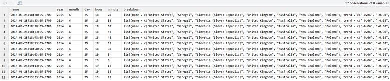
As part of the overall concept of my RSiteCatalyst package, I’m trying to make it as easy as possible for digital analysts to get their data via the Adobe Analytics API. As such, I abstract away the need to build JSON to request reports and parse the API answer from JSON to a data frame. Sometimes it’s easy, but sometimes you get something like this:

nested_r_dataframe

In case it’s not clear what’s going on here, fromJSON() from jsonlite returns a data frame as best as it can, but we have a list (of data frames!) nested inside of a column named “breakdown”. There are 12 rows here, but the proper data structure would be to take the data frame inside of ‘breakdown’ and append all of the fields from the original 12 rows, repeating the values down the rows. So something like 72 rows (12 original rows, 6 row data frames inside of the ‘breakdown’ column).

Loop and Accumulate

Because this is such a small data frame, and because *apply functions are too frustrating in most cases, to parse this I went with the tried-and-true loop and accumulate. But instead of immediately getting what I wanted, I got this fantastic R error message:

1
2
3
4
5
6
7
8
9
10
11
12
#Loop over df and accumulate results
parsed_df <- data.frame()
for(i in 1:nrow(df)){
  temp <- cbind(df[i,],breakdown_list[[i]])
  parsed_df <- rbind(parsed_df, temp)
}

There were 12 warnings (use warnings() to see them)
>warnings()
Warning messages:
  1: In data.frame(..., check.names = FALSE) :
  row names were found from a short variable and have been discarded

Row names from a short variable? Off to StackOverflow, the savior of all language hackers, which lets me know I just need to add an argument to my cbind() function. Trying again:

1
2
3
4
5
6
7
8
9
10
11
12
13
#Loop over df and accumulate results
#Adding row.names = NULL fixes error message
parsed_df <- data.frame()
for(i in 1:nrow(df)){
  temp <- cbind(df[i,],breakdown_list[[i]], row.names = NULL)
  parsed_df <- rbind(parsed_df, temp)
}

names(parsed_df)

> names(parsed_df)
 [1] "name"           "year"           "month"          "day"            "hour"           "minute"         "breakdownTotal"
 [8] "name"           "trend"          "counts"

So I successfully created an (84,10)-sized data frame, but cbind() allowed me to name two columns in the data frame “name”! Running ‘parsed_df$name’ at the REPL returns the first instance. So now, I have to use the unstable method of referring to the second ‘name’ column by position number if I want to access it (or, rename it using names() of course). The way I realized this behavior was occurring was that I tried to use plyr::rename and kept changing the name of two columns!

Final Solution

In order to get past my duplicate name issue, I eventually renamed the ‘name’ columns individually by each object, prior to cbind():

1
2
3
4
5
6
7
8
9
10
11
12
13
14
#Separate breakdown list and original data frame into different objects
df <- ex_df$report$data
breakdown_list <- df$breakdown
df$breakdown <- NULL

#Loop over df and accumulate results
parsed_df <- data.frame()
for(i in 1:nrow(df)){
  right_df <-  breakdown_list[[i]]
  right_df <- rename(right_df, replace=c("name" = report_raw$report$elements$id[2]))
  temp <- cbind(df[i,],right_df, row.names = NULL)
  parsed_df <- rbind(parsed_df, temp)
}
parsed_df <- rename(parsed_df, replace=c("counts" = report_raw$report$metrics$id))

In the end, I found an answer to my solution, but it seems like every time I use R the more oddities I’m able to encounter/generate. At this point, I’m starting to question whether I really understand the underpinnings of how R works. It might be time to stop trying to be a language polyglot so much and focus on really learning a few of these tools in-depth.

Using Julia As A "Glue" Language

Randy Zwitch × June 24, 2014 × DataScience

While much of the focus in the Julia community has been on the performance aspects of Julia relative to other scientific computing languages, Julia is also perfectly suited to ‘glue’ together multiple data sources/languages. In this blog post, I will cover how to create an interactive plot using Gadfly.jl, by first preparing the data using Hadoop and Teradata Aster via ODBC.jl.

The example problem I am going to solve is calculating and visualizing the number of airplanes by hour in the air at any given time in the U.S. for the year 1987. Because of the structure and storage of the underlying data, I will need to write some custom Hive code, upload the data to Teradata Aster via a command-line utility, re-calculate the number of flights per hour using a built-in Aster function, then using Julia to visualize the data.

Step 1: Getting Data From Hadoop

In a prior set of blog posts, I talked about loading the airline dataset into Hadoop, then analyzing the dataset using Hive or Pig. Using ODBC.jl, we can use Hive via Julia to submit our queries. The hardest part of setting up this process is making sure that you have the appropriate Hive drivers for your Hadoop cluster and credentials (which isn’t covered here). Once you have your DSN set up, running Hive queries is as easy as the following:

1
2
3
4
5
6
7
8
9
10
11
12
13
14
15
16
17
18
19
20
21
22
23
using ODBC

#Connect to Hadoop cluster via Hive (pre-defined Windows DSN in ODBC Manager)
hiveconn = ODBC.connect("Production hiveserver2"; usr="your-user-name", pwd="your-password-here")

#Clean data, return results directly to file
#Data returned with have origin of flight, flight takeoff, flight landing and elapsed time
hive_query_string =
"select
origin,
from_unixtime(flight_takeoff_datetime_origin) as flight_takeoff_datetime_origin,
from_unixtime(flight_takeoff_datetime_origin + (actualelapsedtime * 60)) as flight_landing_datetime_origin,
actualelapsedtime
from
(select
origin,
unix_timestamp(CONCAT(year,\"-\", month, \"-\", dayofmonth, \" \", SUBSTR(LPAD(deptime, 4, 0), 1, 2), \":\", SUBSTR(LPAD(deptime, 4, 0), 3, 4), \":\", \"00\"))  as flight_takeoff_datetime_origin,
actualelapsedtime
from vw_airline
where year = 1987 and actualelapsedtime > 0) inner_query;"

#Run query, save results directly to file
query(hive_query_string, hiveconn;output="C:\\airline_times.csv",delim=',')

In this code, I’ve written my query as a Julia string, to keep my code easily modifiable. Then, I pass the Julia string object to the query() function, along with my ODBC connection object. This query runs on Hadoop through Hive, then streams the result directly to my local hard drive, making this a very RAM efficient (though I/O inefficient!) operation.

Step 2: Shelling Out To Load Data To Aster

Once I created the file with my Hadoop results in it, I now have a decision point: I can either A) do the rest of the analysis in Julia or B) use a different tool for my calculations. Because this is a toy example, I’m going to use Teradata Aster to do my calculations, which provides a convenient function called burst() to regularize timestamps into fixed intervals. But before I can use Aster to ‘burst’ my data, I first need to upload it to the database.

While I could loop over the data within Julia and insert each record one at a time, Teradata provides a command-line utility to upload data in parallel. Running command-line scripts from within Julia is as easy as using the run() command, with each command surrounded in backticks:

1
2
3
4
5
6
7
8
9
10
11
12
13
14
15
16
17
18
19
20
21
22
23
24
25
26
27
28
29
30
31
32
33
34
35
36
37
38
39
40
#Connect to Aster (pre-defined Windows DSN in ODBC Manager)
asterconn = ODBC.connect("aster01"; usr="your-user-name", pwd="your-password")

#Create table to hold airline results
create_airline_table_statement =
"create table ebi_temp.airline
(origin varchar,
flight_takeoff_datetime_origin timestamp,
flight_landing_datetime_origin timestamp,
actualelapsedtime int,
partition key (origin))"

#Execute query
query(create_airline_table_statement, asterconn)

#Create airport table
#Data downloaded from http://openflights.org/data.html
create_airport_table_statement =
"create table ebi_temp.airport
(airport_id int,
name varchar,
city varchar,
country varchar,
IATAFAA varchar,
ICAO varchar,
latitude float,
longitude float,
altitude int,
timezone float,
dst varchar,
partition key (country))"

#Execute query
query(create_airport_table_statement, asterconn)

#Upload data via run() command
#ncluster_loader utility already on Windows PATH
run(`ncluster_loader -h 192.168.1.1 -U your-user-name -w your-password -d aster01 -c --skip-rows=1 --el-enabled --el-table e_dist_error_2 --el-schema temp temp.airline C:\\airline_times.csv`)

run(`ncluster_loader -h 192.168.1.1 -U your-user-name -w your-password -d aster01 -c --el-enabled --el-table e_dist_error_2 --el-schema temp temp.airport C:\\airports.dat`)

While I could’ve run this at the command-line, having all of this within an IJulia Notebook keeps all my work together, should I need to re-run this in the future.

Step 3: Using Aster For Calculations

With my data now loaded in Aster, I can normalize the timestamps to UTC, then ‘burst’ the data into regular time intervals. Again, all of this can be done via ODBC from within Julia:

1
2
3
4
5
6
7
8
9
10
11
12
13
14
15
16
17
18
19
20
21
22
23
24
25
26
27
28
29
30
31
32
33
34
35
36
37
38
39
#Normalize timestamps from local time to UTC time
aster_view_string = "
create view temp.vw_airline_times_utc as
select
row_number() over(order by flight_takeoff_datetime_origin) as unique_flight_number,
origin,
flight_takeoff_datetime_origin,
flight_landing_datetime_origin,
flight_takeoff_datetime_origin - (INTERVAL '1 hour' * timezone) as flight_takeoff_datetime_utc,
flight_landing_datetime_origin - (INTERVAL '1 hour' * timezone) as flight_landing_datetime_utc,
timezone
from temp.airline
left join temp.airport on (airline.origin = airport.iatafaa);"

#Execute query
query(aster_view_string, asterconn)

#Teradata Aster SQL-H functionality, accessed via ODBC query
burst_query_string =
"create table temp.airline_burst_hour distribute by hash (origin) as
SELECT
*,
\"INTERVAL_START\"::date as calendar_date,
extract(HOUR from \"INTERVAL_START\") as hour_utc
FROM BURST(
     ON (select
        unique_flight_number,
        origin,
        flight_takeoff_datetime_utc,
        flight_landing_datetime_utc
        FROM temp.vw_airline_times_utc
)
     START_COLUMN('flight_takeoff_datetime_utc')
     END_COLUMN('flight_landing_datetime_utc')
     BURST_INTERVAL('3600')
);"

#Execute query
query(burst_query_string, asterconn)

Since it might not be clear what I’m doing here, the burst() function in Aster takes a row of data with a start and end timestamp, and (potentially) returns multiple rows which normalize the time between the timestamps. If you’re familiar with pandas in Python, it’s a similar functionality to resample on a series of timestamps.

Step 4: Download Smaller Data Into Julia, Visualize

Now that the data has been processed from Hadoop to Aster through a series of queries, we now have a much smaller dataset that can be loaded into RAM and processed by Julia:

1
2
3
4
5
6
7
8
9
10
11
12
13
14
15
16
17
18
19
20
21
22
23
#Calculate the number of flights per hour per day
flights_query = "
select
calendar_date,
hour_utc,
sum(1) as num_flights
from temp.airline_burst_hour
group by 1,2
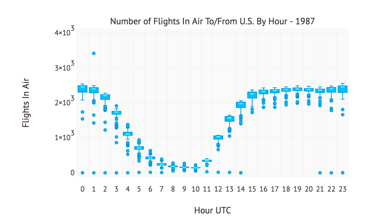
order by 1,2;"

#Bring results into Julia DataFrame
flights_per_day = query(flights_query, asterconn)

using Gadfly

#Create boxplot, with one box plot per hour
set_default_plot_size(20cm, 12cm)
p = plot(flights_per_day , x="hour_utc", y="num_flights",
            Guide.xlabel("Hour UTC"),
            Guide.ylabel("Flights In Air"),
            Guide.title("Number of Flights In Air To/From U.S. By Hour - 1987"),
            Scale.y_continuous(minvalue=0, maxvalue=4000),
            Geom.boxplot)

The Gadfly code above produces the following plot:

gadfly

Since this chart is in UTC, it might not be obvious what the interpretation is of the trend. Because the airline dataset represents flights either leaving or returning to the United States, there are many fewer planes in the air overnight and the early morning hours (UTC 7-10, 2-5am Eastern). During the hours when the airports are open, there appears to be a limit of roughly 2500 planes per hour in the sky.

Why Not Do All Of This In Julia?

At this point, you might be tempted to wonder why go through all of this effort? Couldn’t this all be done in Julia?

Yes, you probably could do all of this work in Julia with a sufficiently large amount of RAM. As a proof-of-concept, I hope I’ve shown that there is much more to Julia than micro-benchmarking Julia’s speed relative to other scientific programming languages. You’ll notice that in none of my code have I used any type annotations, as none would really make sense (nor would they improve performance). And although this is a toy example purposely using multiple systems, I much more frequently use Julia in this manner at work than doing linear algebra or machine learning.

So next time you’re tempted to use Python or R or shell scripting or whatever, consider Julia as well. Julia is just as at-home as a scripting language as a scientific computing language.

« Prev 1 2 3 4 5 6 7 8 9 10 11 12 13 14 15 16 17 18 19 20 21 22 23 24 25 26 27 28 29 30 31 32 33 Next »